Biot-Savart law
QuickField simulation example
Two long wires located at a distance of 100 mm from each other in the air carry opposing currents of 10 A.
Problem Type
Plane-parallel problem of DC magnetics.
Geometry
Given
Currents in conductors I1 = -10 A, I2 = +10 A
Environment - air.
Task
Compute magnetic flux density at the point K.
Solution
The problem can be solved analytically. The value of magnetic flux density according to the Biot-Savart-Laplace law for an infinitely long wire is defined as*:
B = (μ0/4π) * 2*I/r = 10-7 * 2*I/r, where R - is the distance from the axis of the wire.
The flux density vector lies in a plane perpendicular to the current and is directed perpendicular to the radius vector to the point of interest.
At the point K, the flux density vector from the left wire is directed horizontally to the right, and the flux density vector from the right wire is directed to the left downward at an angle (90-63.4)° to the horizontal.
The resulting flux density can be found as a vector sum* of the individual components.
* Magnetic Fields by Superposition.
Result
Magnetic flux density at the point K according to the Bio - Savart law:
From left wire, B1 = 10-7 * 2 * 10 / 0.5 = 4 μT, is directed to the right (B1x = 4 μT, B1y = 0).
From right wire, B2 = 10-7 * 2 * 10 / 1.11 = 1.8 μT, is directed left down (B2x = -0.8 μT, B2y = -1.6 μT).
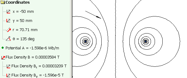
Total flux density, Bx = B1x + B2x = 3.2 μT, By = B1y + B2y = -1.6 μT.
The value of flux density at the point of interest calculated in QuickField and the picture of the vector field of magnetic flux density.
Reference:
* Jackson, John David Classical Electrodynamics. New York: Wiley. Chapter 5.
- Video: Biot-Savart law. Watch on YouTube
- Download simulation files (files may be viewed using any QuickField Edition).