Quadrupole charge
QuickField simulation example
Charges are placed in the vertices of the 1m x 1m square.
Problem Type electrostatics.
Geometry 3D extrusion.
Given
Relative permittivity of air εr = 1,
Electron charge q = 1.602e-19 C.
Quadrupole charges Q1 = 1*q, Q2 = 2*q, Q3 = 3*q, Q4 = -6*q.
Task
Calculate the electric field stress distribution along z axis.
Solution
Analytical solution is based on the equation derived from Coulomb's law*:
E(z) = k * q/R² [V/m], where
k=8.988e9 [N·m² / C²] is a Coulomb's constant,
R - distance from the charge q.
For any arbitrary point on axis z we can find the electric field stress components produced by each charge.
Total electric field stress components are:
Ex(z) = k / r² * cos(β) * (-Q1*cos(α1) - Q2*cos(α2) - Q3*cos(α3) - Q4*cos(α4)),
Ey(z) = k / r² * cos(β) * (-Q1*sin(α1) - Q2*sin(α2) - Q3*sin(α3) - Q4*sin(α4)),
Ez(z) = 0.
where β - elevation angle,
α - angle in the plane XY between vectors O-X and O-charge.
(in our model α1 = 3π/4, α2 = π/4, α3 = -π/4, α4 = -3π/4).
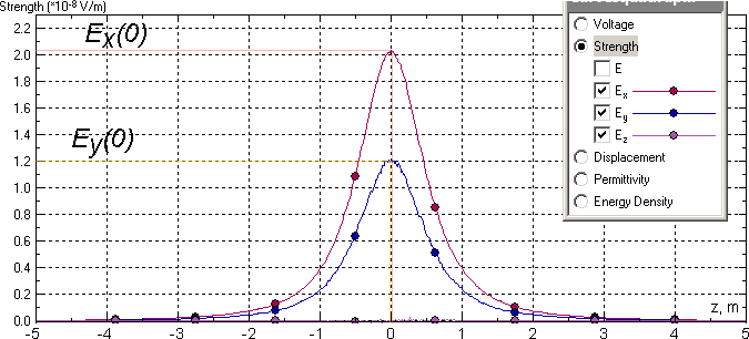
Results
Analytical solution for z=0: cos(β) = 1, R=0.707 m;
Ex(0) = 8.988e9 / (0.707)² * 1 * ( -q*cos(3π/4) - 2q*cos(π/4) - 3q*cos(-π/4) + 6q*cos(-3π/4)) = 1.271e10*(-10q) = 2.04e-8 V/m;
Ey(0) = 8.988e9 / (0.707)² * 1 * ( -q*sin(3π/4) - 2q*sin(π/4) - 3q*sin(-π/4) + 6q*sin(-3π/4)) = 1.271e10*(-6q) = 1.22e-8 V/m;
Ez(0) = 0 V/m.
Electric field stress calculated in QuickField:
*Reference: Coulomb's law in Wikipedia.
- Download simulation files (files may be viewed using any QuickField Edition).