ISO 13786-2017. Periodic thermal transmittance
QuickField simulation example
A homogeneous concrete wall with periodically changing temperature on its surface.
Problem Type
Plane-parallel problem of Transient heat transfer.
Geometry
Given
Thermal conductivity λ = 1.8 W/K-m
Density ρ = 2400 kg/m³
Specific heat capacity C = 1000 J/kg-K
Inner surface resistance Rs_inside = 0.04 m²-K/W,
Outside surface resistance Rs_outside = 0.13 m²-K/W,
Period of thermal variations T=24 hours.
Task
Calculate following parameters and compare them with reference values from ISO 13786:2017:
- periodic penetration depth δ, m
- steady-state thermal transmittance U, W/m²K;
- internal thermal admittance Y11, W/m²K;
- external thermal admittance Y22, W/m²K;
- periodic thermal transmittance Y12, W/m²K;
Solution
Convection coefficient α is used to define the convection boundary condition in QuickField. Convection coefficient is equal to the reciprocal of the heat transfer resistance Rs: α = 1 / Rs.
In QuickField the trigonometric functions arguments are specified in degrees, time is specified in seconds. Sinusoidal temperature can be specified by the sine formula: 1 * sin (2 * 180 * t / 86400), where t is a time variable, T=86400 is a period of thermal variations in seconds. To reach quasi-dynamic state ten periods are simulated, the measurements are made at the last period.
The ISO 13786: 2017 standard defines following conditions for calculating a particular parameter:
- The periodic penetration depth δ is a depth at which the amplitude of the temperature variations is reduced by the factor of e=2.718...
- The steady state thermal transmittance U is defined in ISO 7345 as the heat flow rate [W] in the steady state divided by area [m²] and by the temperature difference [K] between the surroundings on each side of a system:
U = Heat flow rate / Area / Temperature difference. - Thermal admittance Y is the amplitude of the density of heat flow rate on one side resulting from a unit temperature amplitude on the same side, when the temperature amplitude on the other size is zero.
- Periodic thermal transmittance Y12 is amplitude of the density of heat flow rate on one side when the temperature amplitude on that side is zero and there is a unit temperature amplitude on the other side.
Results
| Parameter | QuickField | ISO 13786:2017 | Difference, % |
|---|---|---|---|
| periodic penetration depth δ, m | 0.1425 | 0.144 | 1% |
| thermal transmittance U, W/m²K | 3.557 | 3.56 | <1% |
| internal thermal admittance Y11 | 5.68 W/m²K, time shift 0.93 h. | 5.70 W/m²K, time shift 0.95 h. | 2% |
| external thermal admittance Y22 | 11.54 W/m²K, time shift 1.86 h. | 11.59 W/m²K, time shift 1.87 h. | <1% |
| periodic thermal transmittance Y12=Y21 | 1.83 W/m²K, time shift -5.65 h. | 1.83 W/m²K, time shift -5.68 h. | <1% |
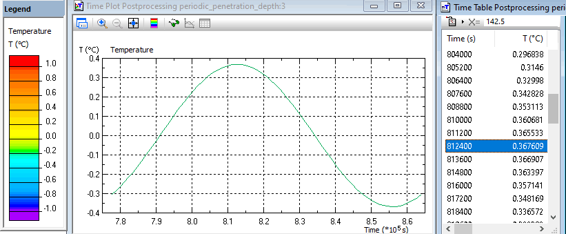
In transient heat transfer problem a temperature boundary condition with sinusoidally changing temperature is applied to a surface of a semi-infinite body. Amplitude of periodic temperature variation is 1 K. At a distance of δ = 0.1425m from the surface the amplitude of a temperature fluctuation is 0.367°C = 1/e. Periodic penetration depth is 0.1425 m.

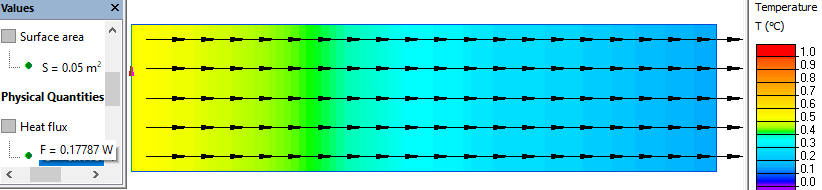
Steady-state heat transfer problem is simulated with convection boundary condition assigned to the opposite wall sides. Air temperature inside is 1°C, air temperature outside is 0°C. Calculated heat flux is 0.1778 W per 0.05 m² of the wall surface area. Steady-state thermal transmittance value is U = 0.1778W/0.05m²/1K = 3.557 W/m²K.
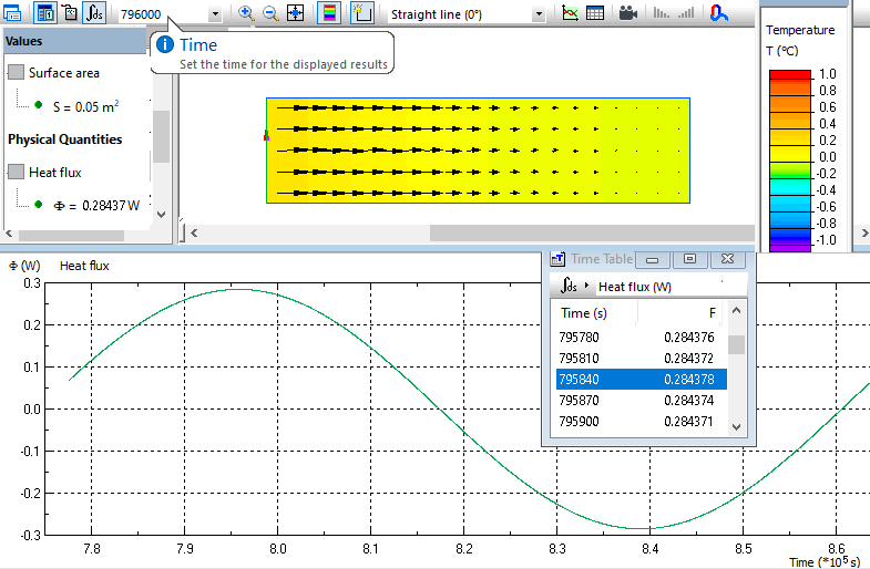
In transient heat transfer problem a convection boundary condition with sinusoidally changing air temperature is applied to the inside surface of the wall. Amplitude of periodic temperature variation is 1 K. At the outside surface convection boundary condition with zero temperature is applied. Ten periods were simulated to reach quasi-dynamic state. Heat flux vs. time is measured at the inside surface. The amplitude of the internal thermal admittance is 0.284W / 0.05m² = 5.68 W/m². The heat flux peak is observed at the moment of time 795840 seconds. The temperature peak occurs at the moment of time (9 + 1/4) * T = 799200 seconds. Time delay between maximum of the heat flux and maximum of the temperature is 799200-795840 = 3360 seconds (0.93 hours).
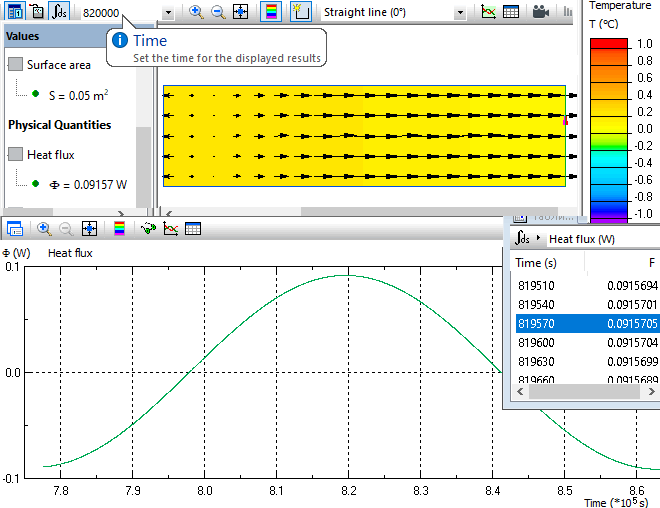
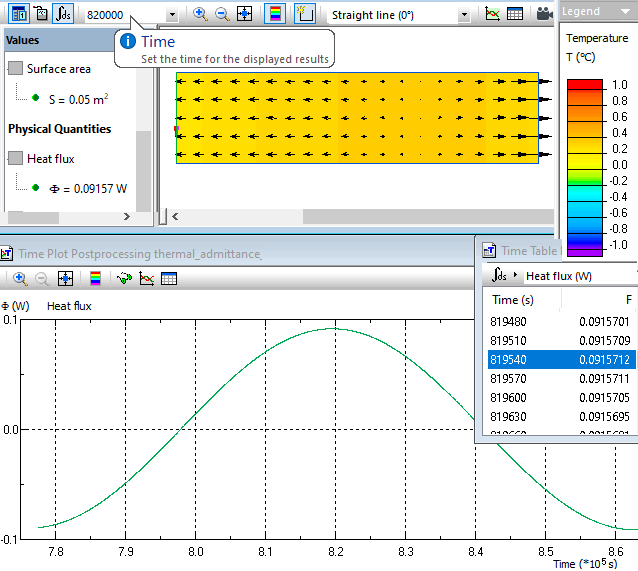
Same heat transfer problem is used to calculate periodic thermal transmittance from the inside Y12. Now the heat flux vs. time is measured at the outside surface. Periodic thermal transmittance at the inside surface amplitude is 0.09157W / 0.05m² = 1.83 W/m². The heat flux peak is observed at the moment of time 819540 seconds. The temperature peak occurs at the moment of time (9 + 1/4) * T = 799200 seconds. Time delay between maximum of the heat flux and maximum of the temperature is 799200-819540 = -20340 seconds (-5.65 hours).
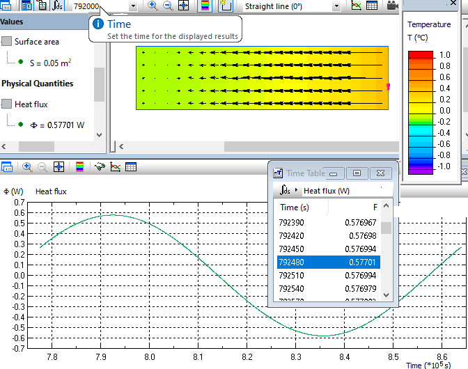
In transient heat transfer problem a convection boundary condition with sinusoidally changing air temperature is applied to the outside surface of the wall. Amplitude of periodic temperature variation is 1 K. At the inside surface convection boundary condition with zero temperature is applied. Ten periods were simulated to reach quasi-dynamic state. Heat flux vs. time is measured at the outside surface. The amplitude of the external thermal admittance is 0.577W / 0.05m² = 11.54 W/m². The heat flux peak is observed at the moment of time 792480 seconds. The temperature peak occurs at the moment of time (9 + 1/4) * T = 799200 seconds. Time delay between the maximum of the heat flux and maximum of the temperature is 799200-792480 = 6720 seconds (1.86 hours).
Same heat transfer problem can be used to calculate periodic thermal transmittance from the outside Y21. Now the heat flux vs. time is measured at the inside surface. Periodic thermal transmittance at the outside surface amplitude is 0.09157W / 0.05m² = 1.83 W/m². The heat flux peak is observed at the moment of time 819540 seconds. The temperature peak occurs at the moment of time (9 + 1/4) * T = 799200 seconds. Time delay between the maximum of the heat flux and maximum of the temperature is 799200-819540 = -20340 seconds (-5.65 hours).
Reference:
* ISO 13786:2017 Thermal performance of building components — Dynamic thermal characteristics — Calculation methods.
- Video: ISO 13786-2017. Periodic thermal transmittance. Watch on YouTube
- Download simulation files (files may be viewed using any QuickField Edition).