Proton E x B Cycloid in Crossed Electric and Magnetic Fields - QuickField simulation example
This example demonstrates how the QuickField Particle Tracer combines independently calculated electrostatic and magnetostatic QuickField solutions to compute the three-dimensional trajectory of a charged particle in combined electric and magnetic fields.
How to calculate the E x B drift cycloid of a charged particle in crossed electric and magnetic fields?
Answer Typical applications Geometry
Given
Task
Solution
Results
References:
A proton starts from rest in uniform crossed fields and follows the classical E × B cycloid. Both QuickField source problems are plane-parallel, but the Lorentz force produces full three-dimensional motion: the trajectory develops in the physical YZ plane while X remains practically constant.
Engineering question
Set up two plane-parallel QuickField problems, Electrostatics and DC Magnetics, for the crossed-field region, then use the QuickField Particle Tracer to combine both fields and trace the proton's cycloidal trajectory and drift velocity.
magnetrons and Hall-effect devices, E × B probes and plasma diagnostics
Download
Simulation problem
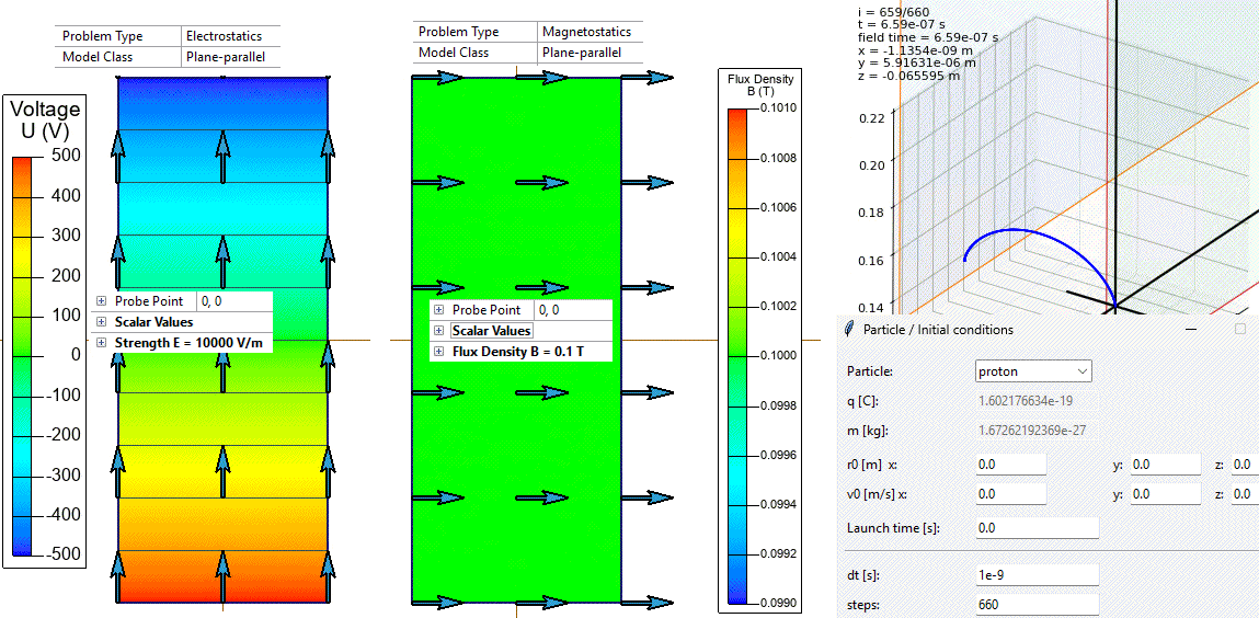
Plane-parallel problems of Electrostatics and DC Magnetics, combined by the Particle Tracer.
Electric field E = (0, +10000, 0) V/m.
Magnetic field B = (+0.1, 0, 0) T.
A proton has charge q = e = +1.6022e-19 C and mass m = 1.6726e-27 kg, starting from rest at the origin.
Calculate the cyclotron frequency and E × B drift velocity, then obtain the proton's three-dimensional cycloidal trajectory over one cyclotron period.
The electrostatic and magnetostatic fields are solved independently as separate plane-parallel QuickField problems.
The QuickField Particle Tracer then combines both field solutions and integrates the equations of motion for the proton under the Lorentz force F = q(E + v × B).
For a particle starting from rest in uniform crossed fields E = (0,E,0), B = (B,0,0), the analytical trajectory is a cycloid*:
y(t) = R· (1 - cos(ωct)), z(t) = -vd· t + R· sin(ωct)
Cyclotron angular frequency: ωc = qB/m = (1.6022e-19 · 0.1) / 1.6726e-27 = 9.5788e6 rad/s
E × B drift velocity: vd = E/B = 10000 / 0.1 = 1.0e5 m/s
Cycloid radius: R = vd/ωc = 1.0e5 / 9.5788e6 = 10.44 mm
Cyclotron period: T = 2π/ωc = 2 · 3.1416 / 9.5788e6 = 655.9 ns
Z drift over one period: ΔZ = -vd· T = -(1.0e5 · 655.9e-9) = -65.59 mm
The proton accelerates in +Y; as its speed grows, the magnetic part of the Lorentz force bends the path toward -Z, producing one cycloidal loop with the expected negative-Z drift.
The X displacement remains below 1 µm throughout, confirming the motion stays in the physical YZ plane.
Over the calculated period the trajectory reaches a maximum Y = 20.88 mm (= 2R) and drifts to ΔZ = -65.60 mm, matching the analytical cycloid.
Quantity
Analytical
QuickField (calculated)
Maximum Y (= 2R), mm
20.88
20.88
Z drift over one period, ΔZ, mm
-65.59
-65.60
* J. B. Tatum. 8.4: Charged Particle in an Electric and a Magnetic Field, Electricity and Magnetism, LibreTexts.
Related examples