High voltage three phase cable ampacity - QuickField simulation example
High voltage 3-phase cable laid in trefoil formation underground.
How to calculate underground three-phase cable ampacity with coupled field simulation?
Answer Typical applications Geometry
Given
Problem:
Solution
Finding out the losses and temperatures distribution is performed in two stages. First the AC magnetic problem is simulated and the results include distribution of the Joule losses, which are then transferred to the Heat Transfer model. Thus for the given electric current in the cable the corresponding temperature distribution is calculated. This is made possible using AC Magnetic to Heat transfer automatic coupling setup in QuickField.
It is possible to take into account the resistivity dependency on temperature. Please refer to the paper above or QuickField Analysis for Electro-Thermal Design webinar.
It is possible to simulate the sheath transposition. Please refer to Transmission line transposition simulation example.
Result
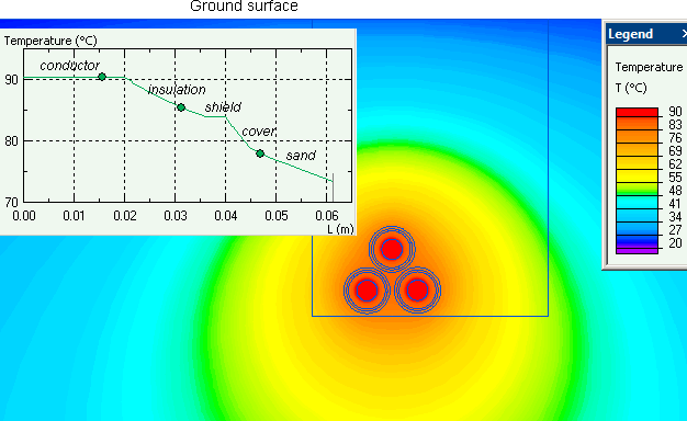
Temperature distribution in the underground cable.
Engineering question
Calculate AC magnetic losses, transfer them to a steady-state heat model, and vary current until the conductor reaches its allowable temperature.
three-phase underground cables, trefoil cable formations, buried HV cable systems
Download
Simulation problem
Problem Type
Plane-parallel multiphysics problem of AC magnetics coupled to Heat Transfer.
The cable system consists of 3 single core cables. Cable line length is 1 km. Shields are ground-connected on both ends.
Current I = 1 kA (RMS), frequency f = 60 Hz.
Air temperature T0 = +20°C, convection coefficient α = 10 W/K*m².
Currents in the cable produce power losses, which heat the cable. Cable ampacity is the current value that leads to the maximum allowable conductor temperature. Therefore, cable ampacity calculation requires simulation of the power losses and temperature distribution for a given current value. This may be considered a practical field-simulation alternative to the analytical methods described in IEC 60287-1-1 and IEC 60287-2-1 [2], [3].
In this example, we determine the losses and temperature distribution for a given current. Then, by increasing or decreasing the current value, we may find the current that corresponds to the maximum allowable conductor temperature — the cable ampacity.
This is a simplified case inspired by the paper: Comparison of Finite Element Analysis to IEC-60287 for Predicting Underground Cable Ampacity by S. Dubitsky, G. Greshnyakov and N. Korovkin presented at ENERGYCON-2016.
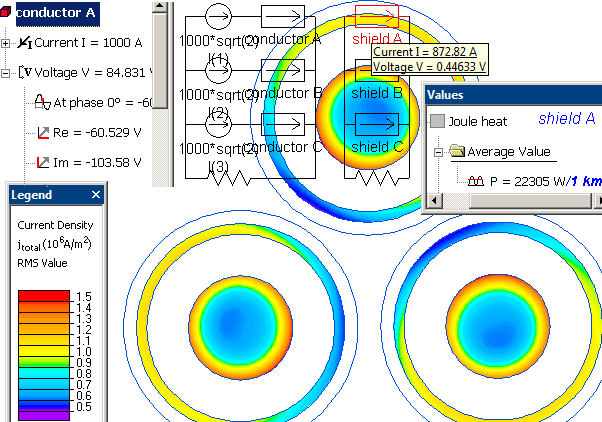
Magnetic field and current density distribution in cable conductor and shield. It could be seen that the electric current density (and Joule loss) distribution is not uniform.
Video
Related examples
References:
[1] IEC 60287:2018 Series. Electric cables - ALL PARTS.
[2] IEC 60287-1-1, Electric cables — Calculation of the current rating — Part 1-1: Current rating equations (100% load factor) and calculation of losses — General, IEC, 2014-11.
[3] IEC 60287-2-1, Electric cables — Calculation of the current rating — Part 2-1: Thermal resistance — Calculation of thermal resistance, Edition 2.0, IEC, 2015-02.